How To Use Vlookup Things To Know Before You Buy
Use VLOOKUP when you require to discover things in a table or a variety by row. For instance, search for a price of an auto component by the part number, or find a staff member name based upon their worker ID. In its simplest type, the VLOOKUP function claims: =VLOOKUP(What you want to seek out, where you desire to try to find it, the column number in the range consisting of the value to return, return an Approximate or Precise match-- showed as 1/TRUE, or 0/FALSE).
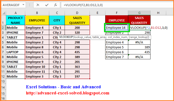
Make use of the VLOOKUP feature to search for a worth in a table. Syntax VLOOKUP (lookup_value, table_array, col_index_num, [range_lookup] As an example: =VLOOKUP(A 2, A 10: C 20,2, TRUE) =VLOOKUP("Fontana", B 2: E 7,2, FALSE) =VLOOKUP(A 2,'Client Facts'! A: F,3, FALSE) Disagreement name Description lookup_value (required) The value you wish to seek out. The value you intend to look up should remain in the very first column of the variety of cells you define in the table_array debate.
Lookup_value can be a value or a recommendation to a cell. table_array (required) The series of cells in which the VLOOKUP will search for the lookup_value and the return value. You can utilize a named range or a table, and also you can utilize names in the debate instead of cell referrals.
The cell range also needs to include the return worth you intend to discover. Discover exactly how to pick ranges in a worksheet. col_index_num (required) The column number (beginning with 1 for the left-most column of table_array) that contains the return value. range_lookup (optional) A rational value that defines whether you want VLOOKUP to locate an approximate or an exact suit: Approximate suit - 1/TRUE thinks the first column in the table is sorted either numerically or alphabetically, as well as will after that look for the closest worth.
As an example, =VLOOKUP(90, A 1: B 100,2, REAL). Exact match - 0/FALSE searches for the precise worth in the very first column. For example, =VLOOKUP("Smith", A 1: B 100,2, FALSE). There are four pieces of info that you will require in order to build the VLOOKUP syntax: The worth you intend to look up, likewise called the lookup worth.
What Does Vlookup Do?
Bear in mind that the lookup worth must always be in the very first column in the variety for VLOOKUP to function appropriately. As an example, if your lookup worth remains in cell C 2 then your variety must start with C. The column number in the variety which contains the return value. As an example, if you define B 2:D 11 as the array, you should count B as the initial column, C as the second, and so on.
If you don't specify anything, the default worth will constantly hold true or approximate match. Now place all of the above together as complies with: =VLOOKUP(lookup value, range including the lookup value, the column number in the variety consisting of the return worth, Approximate suit (REAL) or Exact suit (FALSE)). Below are a few examples of VLOOKUP: Trouble What failed Incorrect worth returned If range_lookup is TRUE or excluded, the first column needs to be sorted alphabetically or numerically.
Either kind the very first column, or utilize FALSE for a precise match. #N/ A in cell If range_lookup is TRUE, then if the value in the lookup_value is smaller sized than the tiniest value in the first column of the table_array, you'll get the #N/ An error worth. If range_lookup is FALSE, the #N/ A mistake value shows that the exact number isn't found.

#REF! in cell If col_index_num is higher than the variety of columns in table-array, you'll obtain the #REF! mistake value. For additional information on settling #REF! mistakes in VLOOKUP, see Just how to correct a #REF! mistake. #VALUE! in cell If the table_array is much less than 1, you'll get the #VALUE! error value.
#NAME? in cell The #NAME? mistake worth normally means that the formula is missing out on quotes. To seek out an individual's name, make sure you make use of quotes around the name in the formula. For instance, enter the name as "Fontana" in =VLOOKUP("Fontana", B 2: E 7,2, FALSE). For more details, see Just how to deal with a #NAME! error.
Examine This Report about Vlookup Formula
Learn how to make use of outright cell recommendations. Don't store number or date values as text. When searching number or day values, be certain the information in the very first column of table_array isn't kept as message values. Or else, VLOOKUP might return a wrong or unexpected value. Arrange the first column Sort the first column of the table_array before making use of VLOOKUP when range_lookup is REAL.
An enigma matches any solitary personality. An asterisk matches any type of series of characters. If you desire to find a real enigma or asterisk, type a tilde (~) before the personality. For instance, =VLOOKUP("Fontan?", B 2: E 7,2, FALSE) will look for all circumstances of Fontana with a last letter that could differ.
When searching text worths in the very first column, ensure the information in the first column does not have leading spaces, routing rooms, irregular use straight (' or") and also curly (' or ") quote marks, or nonprinting personalities. In these instances, VLOOKUP could return an unanticipated value.
You can constantly ask a professional in the Excel Individual Voice. Quick Recommendation Card: VLOOKUP refresher course Quick Recommendation Card: VLOOKUP fixing pointers You Tube: VLOOKUP video clips from Excel area specialists Every little thing you need to find out about VLOOKUP Just how to correct a #VALUE! mistake in the VLOOKUP feature Just how to correct a #N/ An error in the VLOOKUP function Introduction of formulas in Excel Exactly how to stay clear of busted solutions Find mistakes in solutions Excel features (indexed) Excel functions (by classification) VLOOKUP (free preview).
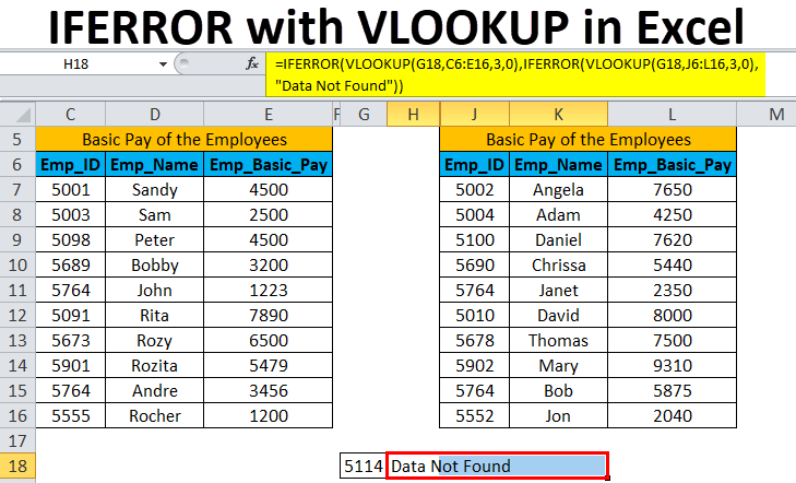
To calculate shipping cost based on weight, you can use the VLOOKUP feature. In the example shown, the formula in F 8 is: =VLOOKUP(F 7, B 6: C 10,2,1)* F 7 This formula makes use of the weight to discover the appropriate "expense per kg" then ... To bypass outcome from VLOOKUP, you can nest VLOOKUP in the IF feature.
vlookup in excel vba array excel vlookup gives #na vlookup function in excel how to use